EXPERIMENT 03 · CONDITIONED ON HAMILTONIAN PARAMETERS DYNAMICS

Two qubits across Hamiltonians.

Exact evolution, MixFunn and conditioned on Hamiltonian parameters temporal continuation.

Symmetric triplet · ℏ = 1

PHYSICAL MODEL AND EVALUATIONExplore this experiment ↓

A family of interacting qubit Hamiltonians

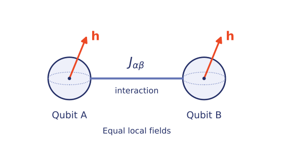
This experiment examines how the quantum trajectory changes with anisotropic qubit interactions. The three diagonal couplings vary independently, while equal local fields remain fixed at h_x = h_y = h_z = 0.5. Evolution begins in |00⟩ with ℏ = 1.

\begin{aligned}H(\mathbf J)={}&\frac12\sum_{\alpha}(\sigma_\alpha^A+\sigma_\alpha^B)\\&+\sum_{\alpha}J_{\alpha\alpha}\sigma_\alpha^A\sigma_\alpha^B.\end{aligned}

Here $\sigma_\alpha^A=\sigma_\alpha\otimes I$ and $\sigma_\alpha^B=I\otimes\sigma_\alpha$ act on Qubit A and Qubit B, respectively; $\alpha,\beta\in\{x,y,z\}$ .

The symmetry under exchange of the two qubits preserves the triplet sector. The neural representation receives (J_xx, J_yy, J_zz, t), so one set of trained parameters describes a family of Hamiltonians. Training samples 512 Hamiltonians in [−1, 1]³ over 0 ≤ t ≤ 4.

Two qubits connected by an interaction, each subject to an equal local field. — Schematic representation. The orange arrows indicate local effective fields. Equal fields on both sites preserve exchange symmetry.

Learning across interaction strengths

MixFunn [1] approximates the complex amplitudes under the Schrödinger equation with supervision from exact observables. The temporal FNO [2] receives the same couplings through additional channels. Its input windows come from MixFunn and its target windows come from exact trajectories. The exact reference was independently checked against QuTiP [3].

Parameters and observables

Changing J_xx, J_yy or J_zz within [−1, 1] recalculates the trajectories with the trained networks. The local fields remain fixed. The graphs display computational basis probabilities, individual Pauli expectation values, diagonal correlators and state fidelity. The viewing interval extends to t = 12, with shading beyond the training horizon t = 4.

Fidelity varies with both the couplings and time. Values across the selected interval quantify accuracy for that Hamiltonian; the sampling range alone provides no bound on the approximation error. Curve visibility and color controls support comparisons throughout the available interval.

Definitions of probabilities, qubit observables and fidelity

INTERACTIVE EXPERIMENT

Parameters and quantum evolution

Back to the physical model ↑

HAMILTONIAN & MODEL

Coupling controls

\begin{aligned}H(\mathbf J)={}&\frac12\sum_{\alpha}(\sigma_\alpha^A+\sigma_\alpha^B)\\&+\sum_{\alpha}J_{\alpha\alpha}\sigma_\alpha^A\sigma_\alpha^B.\end{aligned}

h_x = h_y = h_z = 0.5 Fixed for this experiment

Experiment details

Variable diagonal couplings with fixed symmetric local fields.

Initial state|00⟩

Training time0–4

Evaluation time0–12

Hamiltonians512 · Sobol

The network is conditioned on the three couplings and time. The local fields are fixed; changing them requires a separately trained experiment.

STATE NETWORK4 → 64 → 6Two MixFunn layers · 3,492 parameters

Jxx = 0.13 · Jyy = −0.37 · Jzz = 0.62Loading the trained models…

Time evolution

Observable

ExactMixFunnMixFunn + FNO

Curves and colors

Exact solution

MixFunn

MixFunn + FNO

Shaded region: beyond the training intervalℏ = 1 · time in model units

Mean fidelity · MixFunn—

Minimum fidelity · MixFunn—

Mean fidelity · MixFunn + FNO—

State fidelity

F = |⟨ψ_exact|ψ_model⟩|²

F = 1 denotes identical normalized states up to a global phase.

State snapshot

t = 5.00Training domain

012

F · MixFunn

F · FNO

Norm² · unnormalized MixFunn

Fidelity in the selected interval

Summary statistics are evaluated on 801 uniformly spaced samples of the selected viewing interval. The exact reference remains unchanged when its curve is hidden. Trajectories are interpolated between the 598 evaluation points. Values depend on both the selected couplings and viewing interval.


Method	Mean fidelity	Minimum fidelity	Maximum error 1 − F
MixFunn
MixFunn + FNO

Methods and numerical evaluation

Conditioned on Hamiltonian parameters representation

The Hamiltonian contains variable diagonal interactions J_xx, J_yy and J_zz and fixed fields h_x = h_y = h_z = 0.5. Exchange symmetry restricts the evolution from |00⟩ to the triplet subspace {|00⟩, (|01⟩ + |10⟩)/√2, |11⟩}. Two MixFunn layers [1], with widths 64 and 6, map (J_xx, J_yy, J_zz, t) to the real and imaginary parts of the triplet amplitudes. The first projection includes pairwise input products. The network contains 3,492 parameters and uses sine, cosine and identity functions.

Training domain and supervision

Training uses 512 sampled with a Sobol sequence Hamiltonians in [−1, 1]³ and 200 temporal points on [0, 4]. The objective combines Schrödinger residual, initial condition, normalization and supervised exact observable losses. Optimization uses 550 outer LBFGS epochs. Predictions are normalized before probabilities, correlators and fidelities are evaluated. The parameter box describes the sampling domain; it does not guarantee uniform approximation accuracy throughout that domain.

Fourier operator continuation

The temporal operator follows the temporal FNO approach [2], conditioned on the same three interaction parameters. Its eleven input channels contain six real amplitude components, two sinusoidal positional coordinates and the three couplings. The architecture has three Fourier layers, 32 latent channels and 16 retained modes, totaling 103,110 real parameters. FNO training uses MixFunn input trajectories and exact target trajectories.

Autoregressive inference starts from the first 64 MixFunn samples and advances 32 samples per step, with Δt = 4/199. Predicted amplitudes are normalized, and overlapping output windows are blended before final normalization. The first output window begins near t = 0.643, within the training interval. The next FNO input uses the preceding normalized prediction before overlap blending. Temporal extrapolation, marked by shading, begins at t = 4.

Evaluation and numerical accuracy

The reference is the unitary solution ψ(t) = exp(−iHt)|00⟩, evaluated in the triplet subspace and independently validated against QuTiP. Both neural models are evaluated for each selected coupling triplet; no retraining is performed. The evaluation grid contains 598 points up to t = 12. Displayed curves and instantaneous values use linear interpolation, and the summary statistics use 801 uniformly spaced points within the selected viewing interval. Fidelity is evaluated against the exact state even when the reference curve is hidden.

Fidelity is displayed without performance based filtering. Errors can grow with time and vary across Hamiltonians; successful parameter conditioning does not imply accurate extended temporal evolution. Changing the viewing interval preserves the initial condition at t = 0.

Download experiment configuration

References

Full bibliographic details and scientific background