
Parameterized dynamics of one qubit.
Sparse MixFunn predictions evaluated against exact unitary evolution.
Coherent motion of a single qubit
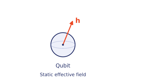
A qubit is a quantum system with two basis states, |0⟩ and |1⟩. A static effective field determines the axis and frequency of its coherent evolution. Here the three field components enter the Hamiltonian through the Pauli matrices, with ℏ = 1 and the initial state |ψ(0)⟩ = |+⟩.
The coefficients hα include the energy scale of the field coupling. With this convention, the Bloch vector precesses around h at angular frequency 2|h|. The exact propagator exp(−iHt) supplies the reference trajectory, independently verified using QuTiP [3].
The three Pauli expectation values form the Bloch vector. A pure qubit state lies on the unit sphere, and its direction determines the state up to a global phase. See [5], [6] and the geometric explanation.
Neural representation
The pruned MixFunn network [1] maps the three field components and time to two complex amplitudes. The two variants use training objectives with or without supervised QuTiP data. Their masks and weights remain fixed during exploration. Probabilities and observables are evaluated after normalizing the predicted state.
Parameters and observables
The field controls vary hx, hy and hz between −1 and 1. The observable selector displays P0, P1 or one of the three Pauli expectations, which are the Cartesian components of the Bloch vector. Fidelity compares the full predicted state with the exact state and is sensitive to relative phase as well as populations.
The time presets extend to t = 10, and the custom interval permits evaluation up to t = 50. Shading identifies times beyond the nominal reference interval [0, 2]. The detailed methods specify how this reference relates to the available training information. Selecting a later viewing interval preserves the preparation at t = 0.
Definitions of probabilities, qubit observables and fidelity
Parameters and quantum evolution
Time evolution
State fidelity
Fidelity is measured against the exact state regardless of curve visibility.
State snapshot
Probabilities and fidelity are evaluated using the normalized state.
Model architecture and sparsity
The parameterized MixFunn representation [1] maps four inputs to two complex state amplitudes through 32 hidden neurons. Binary masks constrain function mixing, input projection and output projection. The dense architecture contains 1,284 parameters; 305 remain active in the supervised variant and 366 in the variant without supervised data.
| Parameter group | Active | Total | Removed |
|---|
The supervised variant removes 90% of input projection coefficients and 39.84% of output projection coefficients. The corresponding fractions without supervised data are 85% and 29.69%. Both variants retain one of three function mixing coefficients per hidden neuron. Model parameters and sparsity patterns remain fixed throughout evaluation.
Methods, reference solution and evaluation domain
Hamiltonian and exact propagator
A single qubit evolves under H = hₓσₓ + hᵧσᵧ + hzσz, with ℏ = 1 and initial state |+⟩. For a static field, the reference state is ψ(t) = exp(−iHt)|+⟩. The analytic propagator is evaluated directly and has been independently checked against QuTiP sesolve for seven Hamiltonians, including H = 0, over [0, 50].
Parameterized neural representation
The MixFunn architecture [1] uses mixed activation functions and second order input features. The input vector (hₓ, hᵧ, hz, t) is augmented by its six distinct pairwise products, excluding individual squares. Sine, cosine and identity functions form the nonlinear basis. Variant specific masks enforce sparsity in function mixing and in the input and output projections. The four outputs encode the real and imaginary components of the two state amplitudes.
Domain and statistical interpretation
Field components vary continuously within [−1, 1]. The nominal sampling grid consists of nine values per axis: −1, −0.75, −0.5, −0.25, 0.01, 0.25, 0.5, 0.75 and 1, giving 729 Hamiltonians. Intermediate fields assess parameter interpolation. The interval [0, 2] is used as a temporal reference; the shaded region marks evaluation beyond this interval. This boundary does not certify the complete temporal coverage of all fine tuning stages.
Probabilities, Pauli expectations and fidelity are computed from normalized states. The unnormalized squared norm is reported separately. Mean and minimum fidelities use 801 samples in the selected interval for the selected Hamiltonian; they do not constitute an aggregate assessment over the full Hamiltonian family. Changing the displayed interval preserves the initial condition at t = 0.