Qubits & geometry MixFunn Temporal FNO Observables Experiments

QUANTA UFSCAR · QUANTUM DYNAMICS

Neural representations of
coherent quantum evolution

MixFunn state representations and Fourier neural operators for interacting spins.

Introduction

Coherent spin dynamics provides a controlled setting for studying neural approximations to the Schrödinger equation. This platform examines a single qubit in a static field and two interacting qubits in the symmetric triplet sector. The experiments compare exact evolution with learned complex amplitudes, assess temporal continuation and explore the dependence of the trajectory on Hamiltonian parameters.

MixFunn combines trainable mixtures of elementary functions with features that include products of input coordinates [1]. The representations used here employ sine, cosine and identity functions. A temporal Fourier neural operator extends selected trajectories through successive windows using a formulation for quantum spin dynamics [2]. Exact references and independent checks with QuTiP provide a common basis for evaluation [3].

01 / QUANTUM SYSTEMS

States, geometry and coherent evolution

Qubit states

A qubit is a quantum system whose state space has two complex dimensions. Choosing orthonormal basis states $|0\rangle$ and $|1\rangle$ gives the expansion below. The complex amplitudes determine measurement probabilities and interference through their relative phase. Normalization fixes the total probability to one; multiplication of the entire state by a common phase leaves physical predictions unchanged [5].

\begin{aligned}|\psi\rangle&=\alpha|0\rangle+\beta|1\rangle,\\|\alpha|^2+|\beta|^2&=1.\end{aligned}

The computational basis outcomes have probabilities $P_0=|\alpha|^2$ and $P_1=|\beta|^2$ . In a spin realization, these states can be chosen as the two projections along a quantization axis. The spin quantum number is $s=\tfrac12$ and the spin operators are $S_\alpha=\hbar\sigma_\alpha/2$ . Throughout this platform, $\sigma_\alpha$ denotes a Pauli operator and Hamiltonian coefficients incorporate the chosen energy convention.

Bloch sphere

A normalized pure qubit state is specified, up to a global phase, by two real parameters. These parameters can be expressed as polar and azimuthal angles on the Bloch sphere, whose Cartesian coordinates are the expectation values of the three Pauli operators [6].

\begin{aligned}|\psi(\theta,\phi)\rangle&=\cos\frac{\theta}{2}|0\rangle+e^{i\phi}\sin\frac{\theta}{2}|1\rangle,\\\mathbf r&=(\sin\theta\cos\phi,\ \sin\theta\sin\phi,\ \cos\theta),\\r_\alpha&=\langle\psi|\sigma_\alpha|\psi\rangle.\end{aligned}

Bloch sphere with computational basis poles, Cartesian axes and a pure state vector r parametrized by polar angle theta and azimuthal angle phi. — **Figure 1.** Geometry of a pure qubit state. The poles correspond to the computational basis; the equator contains equal probability superpositions. The orange vector specifies a state through its direction.

The sphere represents the geometry of quantum states. Its north and south poles correspond to $|0\rangle$ and $|1\rangle$ , while $|+\rangle=(|0\rangle+|1\rangle)/\sqrt2$ lies on the positive x axis. A density operator extends the representation to statistical mixtures. Pure states occupy the surface; mixed states lie inside the Bloch ball, and its center is the maximally mixed state [6].

\rho=\frac{I+\mathbf r\cdot\boldsymbol\sigma}{2},\qquad |\mathbf r|\leq1.

Single qubit dynamics in a static field

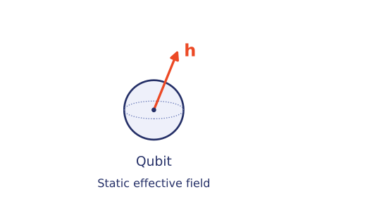
The single qubit experiment begins in $|+\rangle$ and evolves under a static effective field. In units with $\hbar=1$ , the Hamiltonian and Schrödinger equation take the following form.

H=\mathbf h\cdot\boldsymbol\sigma=h_x\sigma_x+h_y\sigma_y+h_z\sigma_z

\begin{aligned}i\frac{\partial}{\partial t}|\psi(t)\rangle&=H|\psi(t)\rangle,\\|\psi(t)\rangle&=e^{-iHt}|\psi(0)\rangle.\end{aligned}

For this convention the Bloch vector satisfies $\dot{\mathbf r}=2\mathbf h\times\mathbf r$ . The field direction sets the rotation axis and its magnitude sets the angular frequency $2|\mathbf h|$ . Changing the three field components therefore changes both the path and rate of evolution. The experiment compares this exact motion with a neural state representation conditioned on the field and time.

Interacting qubits and exchange symmetry

For two qubits, the joint state belongs to $\mathbb C^2\otimes\mathbb C^2$ and contains four complex amplitudes in the computational basis. Interactions can generate entanglement. The reduced states of A and B each admit a Bloch vector, while correlations between them are encoded in the joint density operator. A pure entangled state can thus have local Bloch vectors inside the ball [5].

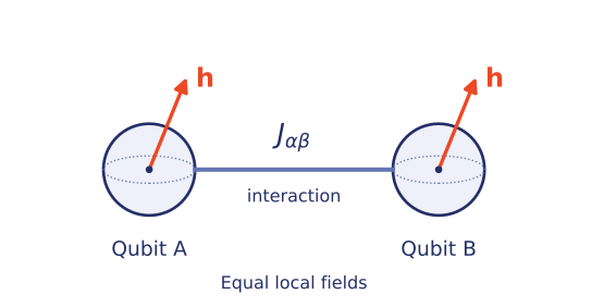
Qubit A and Qubit B with equal local fields h and a coupling tensor J connecting them. — **Figure 2.** Schematic of the two interacting subsystems, labelled A and B. Orange arrows denote effective fields and the connecting line denotes the interaction. Each circle identifies a subsystem; the joint quantum state includes their correlations.

The experiments use equal local fields and interactions symmetric under exchange of A and B. Define $\sigma_\alpha^A=\sigma_\alpha\otimes I$ and $\sigma_\alpha^B=I\otimes\sigma_\alpha$ , where $\alpha,\beta\in\{x,y,z\}$ . The full Hamiltonian is

\begin{aligned}H={}&\sum_{\alpha}h_\alpha(\sigma_\alpha^A+\sigma_\alpha^B)\\&+\sum_{\alpha}J_{\alpha\alpha}\sigma_\alpha^A\sigma_\alpha^B\\&+\sum_{\alpha<\beta}J_{\alpha\beta}(\sigma_\alpha^A\sigma_\beta^B+\sigma_\beta^A\sigma_\alpha^B).\end{aligned}

The first term describes the local fields. Diagonal couplings connect equal spin components, and the remaining terms connect different components symmetrically. Exchange symmetry preserves the three dimensional triplet sector. Evolution from $|00\rangle$ can therefore be represented by three complex amplitudes:

\begin{aligned}|T_+\rangle&=|00\rangle,\qquad |T_-\rangle=|11\rangle,\\|T_0\rangle&=\frac{|01\rangle+|10\rangle}{\sqrt2},\\|\psi(t)\rangle&=\sum_{m\in\{+,0,-\}}a_m(t)|T_m\rangle.\end{aligned}

This symmetry reduction is used in both the fixed Hamiltonian experiment and the family with variable diagonal couplings. The latter keeps the local fields fixed and varies $J_{xx},J_{yy},J_{zz}$ , allowing one trained representation to be evaluated across a continuous parameter domain.

02 / NEURAL STATE REPRESENTATION

MixFunn and the dynamical constraints

MixFunn architecture

MixFunn introduces neurons that combine several parameterized functions with learned mixing coefficients. It also incorporates products of input coordinates to represent interactions between variables. These components provide a flexible function basis for differential equations [1]. Schematically, a mixed function unit has the form

a_j=\sum_{q=1}^{Q}p_{jq}\,f_q(s_{jq}),\qquad s_{jq}=\mathbf w_{jq}^{\mathsf T}\boldsymbol\Phi(\mathbf x)+b_{jq}.

Here $\boldsymbol\Phi$ denotes the input features, $s_{jq}$ is a trainable projection and $p_{jq}$ controls the contribution of each function. The present experiments use sine, cosine and identity functions. Their arguments and mixing coefficients are learned during optimization, allowing oscillatory and slowly varying contributions to share a representation.

For the Hamiltonian conditioned models, the input coordinates contain time and the variable Hamiltonian parameters. Their feature expansion includes the original coordinates and products between distinct coordinates:

\boldsymbol\Phi(\mathbf x)=\bigl(x_1,\ldots,x_d,\{x_ix_j\}_{i<j}\bigr).

With four inputs this gives ten features. Products between a Hamiltonian coefficient and time can encode their joint influence on the evolving amplitudes. Subsequent layers map the hidden features to real and imaginary components of the state: four real outputs for one qubit and six for the triplet representation. The fixed Hamiltonian model receives time alone. The sparse single qubit variants additionally use pruning masks to retain selected trained connections.

Schrödinger residual and training objective

Let $\psi_\vartheta(t;\boldsymbol\lambda)$ denote the neural state, where $\vartheta$ collects network parameters and $\boldsymbol\lambda$ collects Hamiltonian coefficients. Automatic differentiation provides its time derivative. The Schrödinger residual evaluated at sampled times enters the training objective as a dynamical constraint [4].

\mathcal R_\vartheta=i\,\partial_t\psi_\vartheta-H(\boldsymbol\lambda)\psi_\vartheta.

\begin{aligned}\mathcal L={}&w_r\langle\|\mathcal R_\vartheta\|^2\rangle\\&+w_0\langle\|\psi_\vartheta(0)-\psi_0\|^2\rangle\\&+w_n\langle(\|\psi_\vartheta\|^2-1)^2\rangle\\&+w_d\mathcal L_{\mathrm{data}}.\end{aligned}

This expression summarizes the roles of the dynamical, initial state, normalization and supervised terms. Brackets denote averages over the relevant training samples; the weights determine their relative contributions. Individual experiments specify the actual loss terms and weights. The supervised term compares selected predictions with reference data. Training without supervised data sets its weight to zero while retaining constraints from the known Hamiltonian and preparation.

After training, a direct evaluation of MixFunn gives the amplitudes at the requested coordinates. Accuracy outside the sampled domain must be assessed against the exact solution. The normalization used to display observables removes the overall amplitude scale, so the raw squared norm is retained separately as a diagnostic.

03 / TEMPORAL CONTINUATION

Fourier neural operators

Spectral operator representation

A neural operator learns a transformation between functions. The Fourier neural operator parameterizes the nonlocal component of this transformation in Fourier space [7]. A lifting map first embeds the input into hidden channels. Each layer combines a learned spectral transformation with a local linear map and a nonlinear activation. A projection then returns the desired output channels.

\begin{aligned}v_0(\tau)&=P(u(\tau)),\\v_{\ell+1}(\tau)&=g\!\left(W_\ell v_\ell(\tau)+\mathcal K_\ell[v_\ell](\tau)+b_\ell\right),\\\mathcal K_\ell[v]&=\mathcal F^{-1}\!\left[R_\ell(k)\,\mathcal F[v](k)\right],\\\widehat u(\tau)&=Q(v_L(\tau)).\end{aligned}

The transform $\mathcal F$ acts along the sampled window. Learned matrices $R_\ell(k)$ mix channels at retained Fourier modes, while $W_\ell$ acts locally at each sample. The inverse transform combines information across the window. The retained modes control the spectral representation; hidden width and depth control the internal channel capacity and number of transformations [7].

Temporal continuation of quantum states

Temporal Fourier neural operators approximate quantum spin evolution by learning transformations between trajectory windows, enabling evaluation beyond the training interval [2]. The experiments here use a temporal adaptation in which a sampled amplitude window is mapped to a shifted window. Complex amplitudes are represented by separate real and imaginary channels. Positional information is supplied along the temporal grid, and the model with variable couplings also receives the Hamiltonian parameters.

\begin{aligned}u_n&=\{\psi(t_n+j\Delta t)\}_{j=0}^{M-1},\\\widehat u_{n+s}&=\mathcal G_\eta(u_n;\boldsymbol\lambda),\qquad t_{n+s}=t_n+s\Delta t.\end{aligned}

The window length $M$ and shift $s$ determine how successive predictions overlap. A MixFunn trajectory supplies the initial window. Predicted samples are reused for continuation, and overlapping segments are combined by the reconstruction procedure. The displayed temporal grid is tied to each trained model and its evaluation protocol.

For the fixed Hamiltonian experiment, both the input and target windows used to train the temporal FNO are generated from MixFunn. For the model with variable couplings, MixFunn inputs are paired with exact targets. These protocols establish different learning objectives and are identified on their respective experiment pages. Physical penalties used in training complement the window matching objective.

Repeated application propagates both the learned dynamics and any accumulated approximation error. Consequently, the viewing horizon is an evaluation choice whose reliability is measured through agreement with exact evolution, state fidelity and normalization. A longer plotted trajectory alone does not establish accuracy over that interval.

Observables and interpretation

Computational basis probabilities give the distribution of outcomes of a measurement in the chosen basis. Spin expectations describe individual components, and correlators characterize joint measurements. All of these quantities are evaluated from normalized states.

\begin{aligned}P_b(t)&=|\langle b|\psi(t)\rangle|^2,\\\langle O\rangle_t&=\langle\psi(t)|O|\psi(t)\rangle,\\C_{\alpha\alpha}(t)&=\langle\psi(t)|\sigma_\alpha\otimes\sigma_\alpha|\psi(t)\rangle.\end{aligned}

For one qubit, ⟨σ_x⟩, ⟨σ_y⟩ and ⟨σ_z form the Bloch vector. For two qubits, XX, YY and ZZ denote the corresponding diagonal correlators. These expectations lie between −1 and 1. Correlations may contain both classical and quantum contributions, and an entanglement claim requires an additional criterion.

F(t)=\left|\langle\psi_{\mathrm{exact}}(t)|\psi_{\mathrm{model}}(t)\rangle\right|^2.

State fidelity lies between zero and one. A value of one identifies the same pure state up to a global phase. Because fidelity depends on the full state, it can reveal relative phase errors that remain hidden in a single probability curve. The reported mean and minimum refer to the selected sampling interval and Hamiltonian.

The shaded region identifies times beyond the stated training or reference interval. Accuracy in this region is assessed from the comparison with the exact solution. Selecting a viewing interval changes the portion of the trajectory on display while preserving its preparation at t = 0. Color and visibility controls support comparison, and the download controls export figures together with numerical values and the selected parameters.

Experiments

The three experiments progress from a single qubit in a variable field to two interacting qubits with fixed or variable couplings. Each page introduces its Hamiltonian and evaluation protocol before the interactive results.

One qubit across Hamiltonians

Vary the three field components and compare sparse MixFunn representations with exact evolution.

Two qubits with temporal continuation

Compare training with and without supervised data for a fixed Hamiltonian, including MixFunn and FNO trajectories.

Two qubits with variable couplings

Explore J_xx, J_yy and J_zz with fixed local fields and evaluate continuation across Hamiltonians.

References

Farias, T. de S., de Lima, G. G., Maziero, J. & Villas-Boas, C. J. MixFunn: A Neural Network for Differential Equations with Improved Generalization and Interpretability. arXiv 2503.22528 (2025). doi:10.48550/arXiv.2503.22528.
Shah, F., Patti, T. L., Berner, J., Tolooshams, B., Kossaifi, J. & Anandkumar, A. Fourier neural operators for learning dynamics in quantum spin systems. Communications Physics 9, 226 (2026). doi:10.1038/s42005-026-02644-1.
Lambert, N. et al. QuTiP 5: The Quantum Toolbox in Python. Physics Reports 1153, 1–62 (2026). doi:10.1016/j.physrep.2025.10.001.
Raissi, M., Perdikaris, P. & Karniadakis, G. E. Physics-informed neural networks: A deep learning framework for solving forward and inverse problems involving nonlinear partial differential equations. Journal of Computational Physics 378, 686–707 (2019). doi:10.1016/j.jcp.2018.10.045.
Nielsen, M. A. & Chuang, I. L. Quantum Computation and Quantum Information. 10th anniversary edition. Cambridge University Press (2010). Chapters 1 and 2.
Preskill, J. Lecture Notes for Ph219/CS219: Quantum Information. Chapter 2, Foundations I: States and Ensembles. California Institute of Technology (2015). Sections 2.2 and 2.3.
Li, Z., Kovachki, N., Azizzadenesheli, K., Liu, B., Bhattacharya, K., Stuart, A. & Anandkumar, A. Fourier Neural Operator for Parametric Partial Differential Equations. arXiv 2010.08895 (2020; revised 2021). doi:10.48550/arXiv.2010.08895.