EXPERIMENT 02 · SYMMETRIC SUBSPACE

Quantum dynamics of two qubits.

Exact evolution, neural approximation and Fourier operator continuation.

MixFunn · FNO · exact solution

PHYSICAL MODEL AND EVALUATIONExplore this experiment ↓

Interacting spins in the symmetric sector

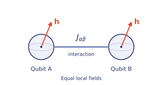
Two qubits experience equal local fields and a symmetric interaction tensor. The local terms rotate each spin, while the interaction terms can generate correlations and entanglement. The initial state is |00⟩ and ℏ = 1.

\begin{aligned}H={}&\sum_{\alpha}h_\alpha(\sigma_\alpha^A+\sigma_\alpha^B)\\&+\sum_{\alpha}J_{\alpha\alpha}\sigma_\alpha^A\sigma_\alpha^B\\&+\sum_{\alpha<\beta}J_{\alpha\beta}(\sigma_\alpha^A\sigma_\beta^B+\sigma_\beta^A\sigma_\alpha^B).\end{aligned}

Here $\sigma_\alpha^A=\sigma_\alpha\otimes I$ and $\sigma_\alpha^B=I\otimes\sigma_\alpha$ act on Qubit A and Qubit B, respectively; $\alpha,\beta\in\{x,y,z\}$ .

Exchange symmetry preserves the triplet basis {|00⟩, (|01⟩ + |10⟩)/√2, |11⟩}. Three complex amplitudes therefore determine the state throughout the evolution. The fields are (0.50, 0.51, 0.49), the diagonal couplings are (0.20, 0.21, 0.19), and (J_xy, J_xz, J_yz) = (0.05, 0.06, 0.04).

Two qubits connected by a spin interaction, each subject to an equal local field. — Schematic representation. The orange arrows indicate local effective fields. Equal fields on both sites preserve exchange symmetry.

Neural representation and temporal continuation

A MixFunn network [1] approximates the triplet amplitudes over 0 ≤ t ≤ 10. The two variants compare training with supervised QuTiP observables and training with physical constraints alone. A Fourier neural operator then advances temporal windows using the approach of Shah et al. [2]. In this experiment, both its input and target windows come from MixFunn trajectories.

Parameters and observables

The controls select the training variant, visible methods, curve colors, observable and viewing interval. The Hamiltonian coefficients remain fixed for these trained networks. Computational basis probabilities resolve the four measurement outcomes. The XX, YY and ZZ correlators describe joint spin measurements along a common axis; a nonzero correlator alone does not establish entanglement.

The fidelity panel compares normalized predicted states with the exact trajectory. Continuation is available to t = 50 for the variant with data and t = 20 for the variant without supervised data. Shading begins at t = 10. The time cursor selects a state snapshot within the chosen interval.

Definitions of probabilities, spin observables and fidelity

Loading model…

Mean fidelity · training domain—MixFunn · t ∈ [0, 10]

Mean fidelity · full interval—MixFunn · t ∈ [0, 50]

Mean fidelity · MixFunn + FNO—Continuation · t ∈ [0, 50]

Time evolution

Observable

ExactMixFunnMixFunn + FNO

Curves and colors

Exact solution

MixFunn

MixFunn + FNO

Shaded region: beyond the training intervalℏ = 1 · time in model units

State fidelity

F = |⟨ψ_exact|ψ_model⟩|²

F = 1 denotes identical normalized states up to a global phase.

State snapshot

t = 5.00Training domain

020

F · MixFunn

F · FNO

Norm² · unnormalized MixFunn

Temporal continuation with FNO

Continuation to t = 50 · fixed parameters

Autoregressive FNO continuation extends the MixFunn trajectory through overlapping temporal windows. Fidelity quantifies agreement with the exact solution throughout the available interval, including times beyond the training domain. The statistics below describe this complete interval and remain independent of the displayed window.

Evaluation over [0, 50], including the training and extrapolation domains.
Method	Mean fidelity	Minimum fidelity	Maximum error 1 − F
MixFunn
MixFunn + FNO

Methods and numerical evaluation

Symmetry reduction and neural representation

The symmetric under exchange Hamiltonian preserves the triplet subspace spanned by |T₊⟩ = |00⟩, |T₀⟩ = (|01⟩ + |10⟩)/√2 and |T₋⟩ = |11⟩. A MixFunn network [1] maps time to the real and imaginary components of these three amplitudes. The 1 → 16 → 6 architecture contains 246 parameters and uses sine, cosine and identity functions. Predicted states are normalized before evaluating probabilities, correlators and state fidelity.

Exact reference and temporal continuation

The reference trajectory is ψ(t) = exp(−iHt)|00⟩, evaluated by spectral decomposition with ℏ = 1. MixFunn optimization uses 4,000 time points on [0, 10] and 50 outer LBFGS epochs. The supervised variant includes a QuTiP observable loss. The variant without supervised data uses the Schrödinger residual, initial condition and norm losses; QuTiP provides an independent evaluation reference. The temporal continuation adopts the temporal neural operator approach studied by Shah et al. [2], adapted here to a hybrid MixFunn and FNO pipeline. MixFunn trajectories provide both the input and target windows for FNO training.

The FNO has three Fourier layers, 32 latent channels and 16 retained modes. Autoregressive inference uses 512 point windows, a 256 point shift and Δt = 10/3999, with blending across overlapping windows. Training combines trajectory error with state normalization, fidelity, Schrödinger residual, overlap and temporal smoothness terms. The available continuation extends to t = 50 for the supervised variant and t = 20 for the variant without supervised data, with fixed parameters in both cases.

Evaluation protocol

The supervised FNO trajectory contains 19,996 time points over [0, 50]. The variant without supervised data is evaluated at 4,000 points over [0, 20]. Displayed FNO observables and fidelities are linearly interpolated between stored samples. Each plot samples the selected interval at 801 points, while the state inspection control evaluates MixFunn directly at the selected time. Full interval summary statistics refer to the selected variant’s complete available interval; the training domain card reports its evaluation within [0, 10]. The two full interval scores cover different horizons and should not be interpreted as a comparison on identical time grids. Changing the displayed interval preserves the initial condition at t = 0. Fidelity is always measured against the exact reference, independently of curve visibility.

References

Full bibliographic details and scientific background